
Correcting Chromatic Aberrations
This is a short howto on determining transverse chromatic aberration (TCA) correction coefficients for use with fulla (a program of the Hugin suite to correct images for distortion, TCA and vignetting) or the Panotools correct plugin. Contrary to other approaches (Krause, PTShift) the approach presented here relies only on free software (Hugin and octave). It is based on automatically creating many control points between the color channels and using these to let PTOptimizer (or another tool) automatically calculate the radial correction parameters.
It is similar to a method proposed by Erik Krause earlier, but according to his words it didn't work very well. This is probably, because the control points were not good enough and/or the images were too colorful.
More information about TCA and its correction using panotools can be found a these webpages:
- A good Introduction by Paul van Walree
- PTShift, photoshop extension for determination of TCA correction coefficients. An alternative way to the approach proposed below. If I had access to photoshop, I would have tried this method first.
- Tutorial by Erik Krause, explains how TCA correction coefficients can be calculated with the help of Picture Window Pro and Excel
Estimating the radial parameters using tca_correct
[April 2008] The Hugin method described below has been superceded by a new tool available with the hugin-0.7.0 release. tca_correct is a command-line program that takes an image file as input and outputs a likely set of fulla correction parameters.
For example, this command will examine a photograph called DSC_1234.tif and generate fulla parameters using the entire a, b, c and d panotools correction model:
tca_correct -o abcv DSC_1234.tif
This level of accuracy is probably unnecessary in most cases, here the c and d panotools parameters should give similar results:
tca_correct -o cv DSC_1234.tif
You can now skip directly to the Correcting TCA section.
Estimating the radial correction parameters using Hugin
- Use a RAW or TIFF photo, trying to correct chromatic aberration of a JPEG photo is a big waste of time. If possible, use an image without much color. Make sure that it not overexposed.
- Split the image into red, green and blue files. This can be done using the decompose filter of the GIMP, or with imagemagick.
- Load them into Hugin, the order should be red, green, blue.
- Give each image a separate 'lens'. Choose equirectangular projection and set the HFOV to 10
- Switch to the Stitcher Tab. Set the Panorama to equirectangular and use a HFOV of 10. Press the "Calculate Optimal Size" button.
- Switch to the Control Points tab. Use the 'g' key to create lots of control points between the green & blue and green & red images. A corner threshold of 50 and a scale of 2 should result in many useful points at corners in the image.
-
Open the preferences and set the fine tune options as in the screenshot below.
Fine tune all points (Edit->Finetune all points). delete any points with less than 98% correlation. This can be done easily with the the control points list. Unfortunately Hugin is very slow when manually selecting many points. Users of Hugin versions later than 10th of March 2006, or 0.6 and higher can use "select by distance" and enter -0.98 to select all points with correlation lower than 0.98
- Optimise FoV and c for the red and blue images. These two parameters are sufficient for most lenses. However, some lenses exhibit a more complicated chromatic aberrations, like the Peleng 8mm fisheye, and require a and b correction parameters as well.
- Delete any bogus control points (with large errors) and reoptimise.
- With any luck you should now have several hundred control-points with an average error of around 0.2 pixels. If not, go back to 8. The preview with blend mode difference can be used to check if the images match well. Mismatches are either caused by overfitting the correction parameters or by color in the input image.
- Save the pto file.
Extracting TCA correction parameters
The distortion parameters of the red and blue channel cannot be used directly by fulla or the PanoTools correct plugin. Therefore I have written an octave script that reads the .pto file, displays the correction curves and provides the parameters for fulla.
The script will also calculate correction parameters based on the control points directly. These might be better than the ones estimated by PTOptimizer.
If you don't have access to octave, here are the formulas and a javascript calculator:
scale = hfov_green / hfov_red

d_pt = 1 - a_pt - b_pt - c_pt
a = a_pt * scale^4
b = b_pt * scale^3
c = c_pt * scale^2
d = d_pt * scale
Use a similar calculation for the blue channel. The values of a_pt, b_pt, c_pt are the distortion parameters from Hugin.
Simple calculator
This calculator uses the output from PTOptimizer to generate the fulla command-line:
If the results are good, then there is no need to try the more complicated octave version below. (Unless you are curious :-)
Download show_tca.m and place it in the same directory as your .pto file. The script requires octave and octave-forge. While I haven't tested if it can be used with MATLAB, it should be useable after slight modifications.
open octave and type:
octave:2> show_tca('pano_tutorial.pto');
This will produce two figures:

This plot shows the scaling factors required for TCA correction of the red and blue channel over the distance from the image center. Each dot represents a control point.
The red and blue line the correction curve estimated by PTOptimizer. The correction curve is also estimated by the show_tca and given by the dotted lines. The correction curves should approximately go through the center of the point clouds.
In my case the values estimated by show_tca look better, since they only depend on the center distance difference (sagittal distance) of the points. PTOptimizer minimizes the tangential and sagittal distance between the points. However, then tangential distance is not of interest for TCA correction, and is caused by the limited accuracy of the fine tune function, especially close the the edge of the fisheye image.

This plot displayes the tangential and sagital distance between the control points of the red and green channel. One can see that there is a significant tangential distance (especially at higher radi), leading to a non-optimal correction coefficients, if PTOptimizer is used.
The calculated correction parameters are printed to the console:
correction parameters read from pto file:
 -r 0.0000000:-0.0019056:0.0030218:0.9995177
 -b 0.0000000:0.0003038:-0.0006342:1.0012401
new fit, based on distance to image center:
 -r 0.0001368:0.0002725:-0.0006605:1.0007630
 -b 0.0011642:-0.0046154:0.0055706:0.9989218
Choose the set of parameters that looks better on the diagram above. I suspect that the second parameter set is usually preferable.
The correction parameters should be useable with all future images shot using the same lens at the same focal length. The correction coefficients will probably vary (a little?) with the focus setting, and maybe even with the aperture (but probably to a lesser degree).
Correcting TCA
The estimated TCA correction coefficients can then be used with fulla or the PanoTools correct plugin.
Correct TCA using fulla:
fulla  -r 0.0001368:0.0002725:-0.0006605:1.0007630 \
       -b 0.0011642:-0.0046154:0.0055706:0.9989218 \
        input.tif
This correction can be combined with all other correction options of fulla, like the distortion correction based on the PTLens database (-p option) or the vignetting correction.
Results
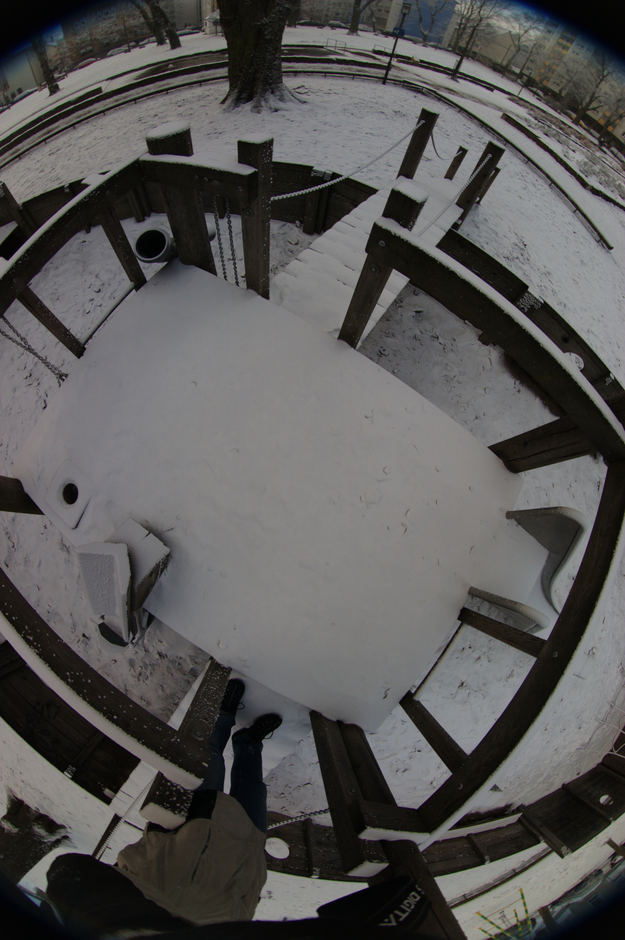
Here are some results of the correction of 8mm Peleng fisheye, used on a Canon 300D:

Correction results near the image corner. The color seams are corrected well.

Correction results near the image center. The center area doesn't show such less TCA than the edges, but it is still corrected well.
Here are the full resolution images: original corrected
Authors: Pablo d'Angelo and Bruno Postle - Created March 2006